blog.dayflower.org

Path tracing is a variation of a Monte Carlo method-based ray tracing algorithm, that finds a numerical solution to the integral of the rendering equation. If done correctly, this will result in an image that is indistinguishable from a photograph. Both the rendering equation and path tracing were presented by James Kajiya in 1986.

The rendering equation is an integral equation with basis in physics. It follows the law of conservation of energy for radiance; the radiant flux emitted, reflected, transmitted or received by a surface.

By using path tracing, the image will get a lot of effects for free. Some of them are global illumination, reflections, refractions, caustics and color bleeding. Global illumination is direct and indirect illumination. Direct illumination is when light hits a given surface directly, whereas indirect illumination is when light bounces around and finally hits a given surface. Reflections occur when light hits a reflective surface, such as a mirror. Refractions occur when light hits a refractive surface, such as glass, where it enters the surface. Caustics occur when light is concentrated. It happens when light is reflected or refracted by a curved surface. Color bleeding occurs when the color of a surface, or albedo as it is commonly referred to, can be seen on another surface. If one surface is green and another white, you may be able to see a green tint on the white surface.

Normally, when using ray tracing, you’d add lights to your scene to see anything. This is not necessary in path tracing. Any object in the scene can act as an emitter of light. If you add explicit lights, you cannot add point lights because they have no area. The probability to hit a point light would be zero.

A potentially disturbing side-effect of path tracing is noise. The more samples you use, the less noise there will be in the final image. But this takes time. There are many ways to reduce noise, such that less samples are required for approximately the same end result. One way to reduce it, is to use larger light-emitting objects, such as a sky. The probability for a ray to hit a larger object is higher than that of a smaller one.

Just as with ray tracing, there are many variations of path tracing. One is bidirectional path tracing.

This blog post will not cover the exact details for an implementation. But some pseudo code will be posted here below, so you can see the overall picture.

void render() {
    Camera camera = createCamera();
    
    World world = createWorld();
    
    Display display = createDisplay();
    
    Sampler sampler = createSampler();
    
    for(int y = 0; y < display.getHeight(); y++) {
        for(int x = 0; x < display.getWidth(); x++) {
            Color color = Color.BLACK;
            
            for(int sample = 0; sample < SAMPLE_COUNT; sample++) {
                Sample2D sample2D = Sample2D.toExactInverseTentFilter(sampler.sample2D());
                
                Ray ray = camera.newRay(sample2D.u + x, sample2D.v + y);
                
                color = color.add(integrate(ray, world));
            }
            
            color = color.divide(SAMPLE_COUNT);
            
            display.update(x, y, color);
        }
    }
}

Color integrate(Ray ray, World world) {
    int currentDepth = 0;
    
    Ray currentRay = ray;
    
    Color color = Color.BLACK;
    Color radiance = Color.WHITE;
    
    while(currentDepth++ < MAXIMUM_DEPTH) {
        Intersection intersection = world.intersection(currentRay);
        
        if(intersection.isIntersecting()) {
            Primitive primitive = intersection.getPrimitive();
            
            Material material = primitive.getMaterial();
            
            Texture textureEmission = primitive.getTextureEmission();
            
            Color colorEmission = textureEmission.getColorAt(intersection);
            
            color = color.add(radiance.multiply(colorEmission));
            
            Result result = material.evaluate(radiance, currentRay);
            
            radiance = result.getRadiance();
            
            currentRay = result.getRay();
        } else {
            break;
        }
    }
    
    Intersection intersection = world.intersection(currentRay);
    
    if(!intersection.isIntersecting()) {
        color = color.add(radiance.multiply(world.getBackground().radiance(currentRay)));
    }
    
    return color;
}

Using my own renderer, with code similar to the one above, I produced the following image. It took a few seconds to generate, so you may still see some noise in there. But, had I not used a sky, you’d see a lot more noise.

Both image order algorithms and object order algorithms are used for rendering. But what’s the difference?

First of all, lets talk about image order algorithms. These algorithms iterate over the pixels in an image and computes the colors of said pixels. The first example that comes to mind is any of the ray tracing algorithms out there. In addition, these algorithms are pretty well suited for OpenCL.

Now lets look at object order algorithms. They iterate over the objects in the scene and attempts to find out what pixels they occupy in the final image, if any. Once they are known to occupy at least one pixel in the image, the color is computed. One algorithm that does this is a scanline rasterizer. These algorithms are the ones primarily used in DirectX and OpenGL.

So, now that we know the main differences, are there any advantages and disadvantages to either? Yes, there are. Because an image tends to have a lot of pixels, usually more so than there are objects in a scene, a lot of time is wasted iterating over all pixels. Not to mention all intersection tests that are required by ray tracing algorithms. So for realtime graphics, object order algorithms are the preferred way. But, object order algorithms tend to complicate things a lot when it comes to photo-realistic rendering. This is where ray tracing algorithms really shine. For instance, do you want to add reflection, refraction or global illumination? Then, essentially, just send more rays and that will solve the problem.

Ray tracing, as a term, can be found in both computer graphics and physics. However, this blog post will only focus on the computer graphics part of it.

So then, what is ray tracing? Ray tracing is an umbrella term for a wide variety of image order algorithms. An image order algorithm iterates over the pixels in an image to produce it. Contrast that with the object order algorithms, that iterate over the objects in the scene in order to produce the final image. However, this is only half the story. The other half is how to produce the final image.

To produce the final image with ray tracing, a ray is computed for each pixel and sent into the scene. The computation of the ray is based on a virtual camera in the scene and a plane defined by the image itself. When the ray has been sent into the scene, it is tested for intersections with all objects in the scene. If the ray intersects an object, the color of the pixel can be calculated by some shading algorithm. If the ray intersects more than one object, make sure the closest object is used in the shading process. If it did not intersect an object, use a constant color, such as black, or a background image to calculate the color of the pixel.

So what should the shading algorithm do? Its purpose is to calculate the color of the pixel based on an intersection with an object. So it could do as little as return a constant color for a specific object, or it could do a lot more. The sky is the limit. However, a constant color is a good start. Once you’ve come this far, you can add lights to the scene and send so called shadow rays from the intersection point of the object to the lights. If there are no intersections between the two, the light hits the object and thus it can be seen from the virtual camera and shaded accordingly.

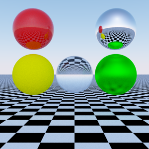
What is described above is often called ray casting. That is, rays sent from the camera into the scene, which are often called primary rays. From here it is possible to create other ray tracing algorithms, such as Whitted ray tracing, which sends secondary rays from the surface intersection point of the object in order to calculate reflections and refractions. There are many more variations out there, some using so called Monte Carlo methods, which essentially sends primary rays in seemingly random directions and calculates an average pixel color.